FMTLab 2026-03-06: How I did it!
What is FMT/FMTLab? 🔗
It is about measuring stuff with higher precision than normally needed. It has little practical value, but can be an interesting intellectual challenge. I’ve certainly learned quite a bit!
So if you are that kind of person, and, after reading the below, some small voice inside tells you: “Oh, this sounds like fun!”, that voice may well be right and I recommend you give it a try!
FMT 🔗
“Frequency Measurement Test”, short FMT, is a traditional radio amateur nerd challenge. To take part, you measure the frequencies of four carriers that are being transmitted for a full minute each, two in the 40 and two in the 80 m band.
The ARRL brings us this fun. Typically, some 50-100 people take part. This happens twice a year. As of this writing, the next competition is to take place April 17, 2026. See the FMT website for details.
The “historical results” there each have a the method/soapbox table. Reading up entries there gives you some idea how such measurements can be done. I find those a fun read, as different people have quite different methods.
If you are that kind of nerd, I can warmly recommend to you: Chose your method and take part! If you are anything like me, you’ll have some good fun and learn a thing or two.
FMTLab 🔗
Recently, a Polish team has appeared on the scene. Under the name “FMTLab”, they take this nerd challenge and carry it a bit further. Same as ARRL, they also challenge you to measure frequencies. But also impulse lengths and, if you are up to it, the timestamp of when impulses get sent. So three challenges total. You can hand in any subset of these three, as you find yourself enticed and able. If you do all three, taking part in FMTLab is a bit more demanding than ARRL’s FMT. But it is still doable for a normal ham, you need not be a specialist.
FMTLab gives you more opportunities: They provide six of what they call “tours” during the first half of 2026 alone, not just two per year as does the ARRL.
Each tour spreads to different times and bands during the same day. You only need to receive and analyze the signal they send on one band (at one time), to take part.
The transmission on one band is roughly 15 minutes long. For the first minute, they send a train of three short impulses, and repeat that train over and over again, once a second, for a minute. Next, they send a carrier for another minute. After that, a short Morse code id, then the whole parcel of 60 x 3 impulses and one minute carrier and Morse code id is repeated, for a total of six times.
FMTLab already offered three tours; the remaining three will happen April 3, May 1, and May 29. For more details, see their web site.
I took part in the February 13 tour and now in the March 6 tour. My March 6 participation is what this blog post is about.
FMTLab is the “new kid on the block”. Not many people know about it yet. (I try to contribute my part to change that.) So not many have jumped on the bandwagon yet. For the March 6 tour, I was one of only seven people who handed in their measurements to the FMTLab web site.
Rest assured my station is nothing special! I have a reasonably stable TRX, but no fancy measurement equipment.
Still, I obtained:
A pleasant result 🔗
My FMTLab measurements March 6, 2026 had errors as follows:
| Challenge | my error |
|---|---|
| Frequency measurement 80 m band | -0.184 Hz |
| PPS offset | 0.759 ms |
| Pulse length | -0.061 ms |
I’m very pleased to measure a frequency in the 80 m band down to better than one fifth of a Hz, and to determine pulse length and PPS offset (some sort of timestamp, explained in more detail below) to better than 1 ms.
I’m not sure what to think about the spectacular precision of my pulse length measurement. From 360 individual pulses, grab the length with a precision of about 21 sound samples (at 48000 samples per second)? Let’s see to what extend I can repeat such nice results in later experiments.
The following gives some record how I did it.
If you want to take part in FMT or FMTLab yourself, too, you may or may not find this blog post helpful. You’re certainly invited to use any of this material (under the licenses as granted) as far as it fits your style and situation. On the other hand, this blog post is mostly intended to documented how I did it, not so much to be reproducible by most other people.
A while ago, I wrote an article on measuring frequencies, with a view of calibrating your rig. That piece is more of a reproducible recipe. That recipe can easily be adopted become a method how to take part in the ARRL FMT and to answer the frequency measurement challenge of FMTLab.
Equipment 🔗
The following is a copy from what I typed into the FMTLab site to describe my equipment, when handing in my results. It is mostly intended for the initiated, who already know what the stuff mentioned is. The others will find a more thorough explanation in later material.
IC-705, T15 Laptop running Debian Trixie with NTP-disciplined clock.
A homegrown C++ program grabs data from the trx’s build-in sound card, writes those as a raw (little-endian 48000 samples-per-second 2 bytes per sample) sound file, and also writes timestamps whenever new samples come in, to a parallel file.
The hard work is done by FLOSS: scipy.signal.ShortTimeFFT and scipy.signal.periodogram and scipy.signal.convolve mostly. For looking into the data, pcolormesh from matplotlib.pyplot helps, and, of course, pandas.DataFrame. Finally, Jupyter notebook provides an environment to harness the other stuff.
A more detailed (and more understandable) record of what I have been doing follows. For those so inclined, the later parts of it even include the files needed to re-run my analysis on your computer.
Method 🔗
The indented quotes that follow together give a copy of what I typed into the FMTLab site to describe my method. When doing so, I was scratching at the maximal length they allow you to enter. Here, in my blog, I can write as long and detailed as I please, and also include pictures.
The first part of what I handed in says:
The 80 m band transmission was again by far the strongest, so I exclusively used that. But I wasn’t able to find the correct frequency until about 2.6 minutes into the transmission, as it deviated considerably from the previously advertised one. So I missed the initial transmission at a well-known frequency. As I had calibrated my rig with the RWM time signal transmitter that day, I hope to be reasonably fine anyway.
Here is a rotated waterfall (x-axis time, y-axis frequency, color codes amplitude) of the entire recording I did:
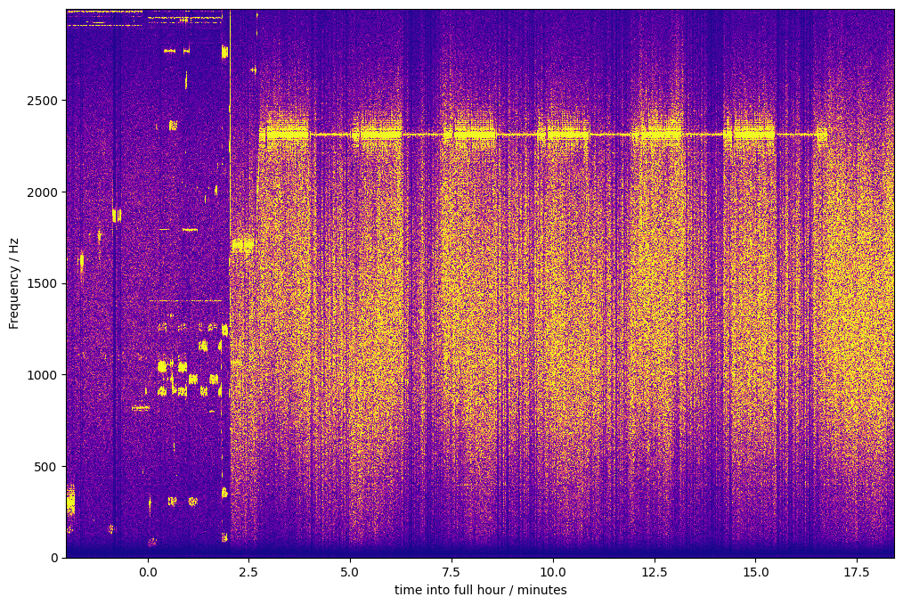
Image description for details and accessibility: The signals visible in this waterfall start with some digital mode signals. At that time, I had the rig’s frequency set to 3567200 Hz. I then moved to 3564000 Hz, and shortly thereafter, to 3563400 Hz, which I reached some time during the minute 21:02 UTC. I reached that frequency early enough so the first batch of pulses had not yet started. After I had reached my final frequency, the waterfall shows a continuous signal at about 2312-2313 Hz. The line that traces that signal becomes thicker and thinner: It is thicker whenever FMTLab sent its Morse code message or its impulse batch. If you look carefully, you can even see the small silent gap between the Morse code and the impulse batch. The line becomes much thinner when the carrier is sent. This is consistent with the smaller bandwidth of a constant carrier, compared to a Morse code or impulse train. After six thick/thin pairs, a shorter thick line segment marks the final Morse code signoff. After that, the signal is gone.
I recorded audio with well-known USB dial frequency, and record timestamps each time a 1024 audio sample batch comes in from the rig.
I was a bit suspicious about those time stamps. My PC’s clock is disciplined by plain NTP, and I’m running the software under Linux, not real-time. So I first looked into those timestamps.
Mostly usable, but a time jump of about 6 ms is visible in the data and raised some concern. Apparently, some 6 ms of samples are missing? This may have occurred when I changed frequency (didn’t bother to verify).
However, I satisfied myself that this jump happened early enough to not matter. It precedes anything that influences my answers to the challenges. So I just ignored that time jump.
My frequency challenge answer 🔗
So here is my answer to the frequency challenge as typed into the FMTLab site:
All error boundaries are just educated guesses.
With FFT from scipy, I found the audio frequency 2312.586 Hz ± 0.1 Hz. My trx was set at USB 3563400 Hz, I estimate its true frequency as 3563399.950 ± 0.5 Hz and allow maybe another ± 0.5 Hz for ionosphere instability. So 3565712.536 Hz ± 1.5 Hz.
Details on how I did this:
The guesstimate that my (well calibrated) TRX is off by some 0.05 Hz in the 80 m band is extrapolated from an analysis of RWM time signal recordings.
That RWM analysis itself I did not bother to publish. The methods used there are rather the same as the ones presented here, even here in this very section.
To find the audio frequency is a two-step process: First, I simply zoom into the same waterfall graph already shown. I zoom to different locations six times, to find the six one-minute carriers. Each zoom magnifies both time-wise and frequency-wise, and I also adjust the colors slightly for good contrast.
Here is one of the six resulting zoom examples:
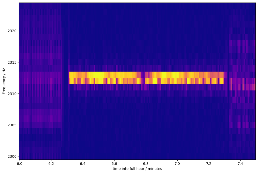
Image description for details and accessibility: This shows a time-wise zoom from 6 to 7.4 minutes after the hour. In y direction, frequencies from 2300 to 2325 Hz are shown. The underlying Fast Fourier Transformation comes up with bins 1 Hz wide. A bright line lasting from about 6.3 to 7.3 minutes stands out clearly. This is one of the one-minute carriers transmitted by FMTLab. Before that line, some weaker, more spread-out signal is dimly visible. That could be the previous impulse batch showing itself. After, some similar signal trace can be seen; that could stem from the Morse code id. The impulse train frequency is hard to estimate due to its high bandwidth; the Morse code id seems to come in at a frequency about 1 Hz below that of the carrier, but this is uncertain (and irrelevant). The bright carrier line spans two bins, corresponding to 2312 and 2313 Hz. Most of the time, the 2313 Hz bin is brighter, but sometimes, the 2312 Hz bin is, in particular around a brief fading incident at about 6.75 minutes into the hour. I guess this reflects changes in ionospheric Doppler shift.
I did not use this zoomed-in waterfall image directly to determine the frequency. But I read from it the time when the 60 second carrier was received. I don’t bother about ultimate time precision here, I only determine an interval of 54 seconds during which the carrier was captured by my recording.
The recording of that entire 54 seconds time interval I feed into
periodogram from scipy.signal. That gives me some spectrogramm
that shows amplitudes vs. frequencies. From what it outputs, some
straightforward code finds the maximum frequency value. Also, for
visual inspection, I plot amplitude over frequency in the interesting
frequency range. Here is one such plot as it appears in my analysis,
amplitude over frequency, for some 54 carrier seconds hand-picked from
the above waterfall zoom picture:
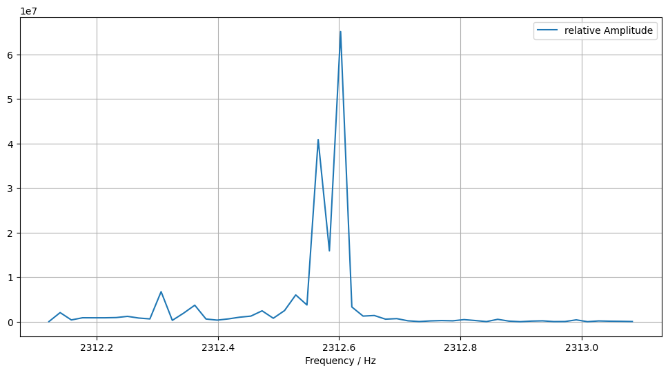
Image description for details and accessibility: This shows a x/y view of the periodogramm. The y-axis shows arbitrary numbers from 0 to 6.5e7, as they happen to be generated by the math underlying the periodogramm. The x-axis shows frequencies between 2312 and 2313 Hz. The graph shows a double peak: One peak is at about 2312.6 Hz with y value roughly 6.2e7, the other at about 2312.58 Hz with smaller y-value, slightly above 4e7. Between them is a valley at roughly 1.6e7. All other values are well below 1e7.
This gives the frequency value of one carrier. The peak values obtained from all six carriers were 2312.6024 Hz, 2312.6024 Hz (this is the one we saw), 2312.5997 Hz, 2312.5274 Hz, 2312.6015 Hz, 2312.5803 Hz. The average of these comes out at 2312.5856 Hz, which, rounded to three decimal places, is the 2312.586 Hz reported.
This concludes the discussion of my frequency measurement.
My pulse length challenge answer 🔗
FMTLab advertises they send six batches of 60 impulse trains each. Each impulse train consists of three impulses. Within each batch, the impulse train is repeated once per second.
The first impulse has a known length of 100 ms, the second of 50 ms. The challenge is to measure the unknown length of the third impulse.
To get started on this one, I manually sifted through my recording and tried to find the first and the last train of each batch. I then let some automated analysis loose on each batch.
I used some kind of oscilloscope plots of the raw recorded data to find the impulse batches. While searching, I used different time-wise zoom levels. Here is one end result of such a search, in four such plots:
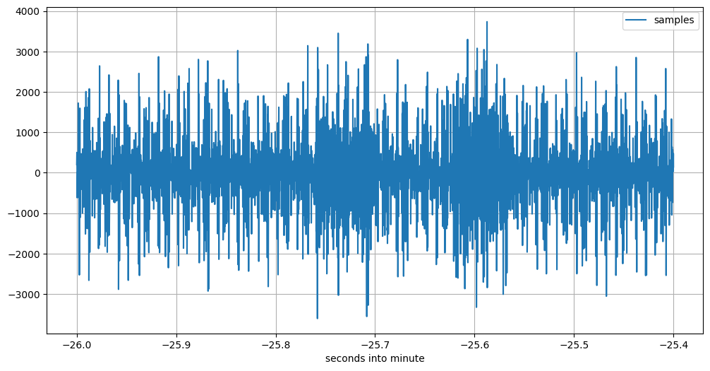
Image description for details and accessibility: This shows the recorded signal for about 0.6 seconds, starting 21:07:34 UTC sharp. The signal contains just noise, with values ranging from 0 to peaks at about -3500 or +3300 with little discernible structure.
One second later, at 21:07:35, it is a different story. This is what one train of three impulses looks like:
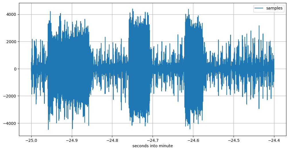
Image description for details and accessibility: This plot, starting 21:07:35 UTC sharp, clearly shows the three impulses as transmitted by FMTLab. The highest peaks in the noise before, between, and after the pulses only occasionally reach slightly above a sample value of 2000 or below one of -2000, while the impulses amplitude rarely are lower than 2000. So the shape of the three impulses clearly comes out.
This is the first three-impulse train in this 60-seconds batch.
After having found the beginning, I search for the end.
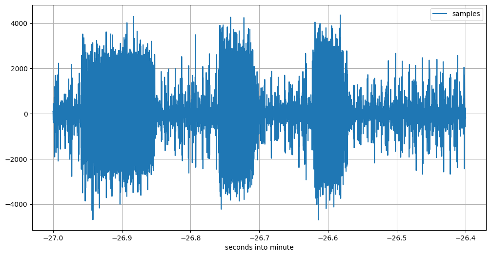
Image description for details and accessibility: This plot, starting 21:08:33 UTC sharp, clearly shows another three impulses as transmitted by FMTLab. The picture itself is similar to the previous one. This is the 59th three-impulse train.
But there should be 60 three-impulse trains. So we need to look yet one more second further:
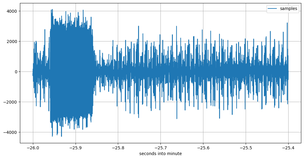
Image description for details and accessibility: This plot, starting 21:08:34 UTC sharp, should show the 60th and last three-impulse train. But it doesn’t. It shows only the first of the three impulses; then noise follows.
I have seen various irregularities with several 60th impulse trains, in this and some of the other batches. I informed the FMTLab team about this, they will look into it.
The first seconds of each impulse batch as I manually dug it out of my data are: 21:02:58 UTC, 21:05:17 UTC, 21:07:35 UTC, 21:09:53 UTC, 21:12:11 UTC, 21:14:29 UTC. From the first to the second impulse batch it is 139 seconds, for all others, it is 138 seconds.
Starting with those listed seconds, I then had some automated code look at 59 three-impulse trains (omitting the last, flaky ones). Here is what I wrote about this when handing in my results:
For the pulse length, I used a convolution each to find the rising and falling edge of each pulse. As far as I can tell, FMTLab did not send the full 360 pulses, but sometimes left out some at end of a pulse minute. For each pulse minute, I determine the median of the pulse length and throw out all pulse lengths that deviate from it by more than 2 ms (QSB). A total of 245 samples survived, the average is 43.239 ms pulse length. I notice that the same way to measure the pulse length of the 100 ms and 50 ms pulses produces values about 1.1 ms too short, so my pulse length value is 44.339 ms ± 2 ms.
Going through my Jupyter notebook again, I find this is actually wrong. What I really did is close, but not quite the same: I determine the median of pulse start and of pulse end separately, both with respect to the start of the pertinent UTC second. I then filter out all pulses when either of the edges is further away from the corresponding median edge by more than 2 ms. Then, I calculate average edges and from there, impulse length.
That concludes the overview how I measured the impulse length.
My PPS offset challenge answer 🔗
Finally, only one challenge is unanswered: It asks you to determine how many milliseconds of delay into its full UTC second does the first impulse of each impulse train start. The FMTLab crew calls this the “PPS offset”, as it can be measured by obtaining the offset between a GPS-device’s pulse-per-second and the start of FMTLab’s initial 100 ms pulse.
From the above pictures, you can check the impulse starts a little less than 50 ms after the full second. But “a little less than 50 ms” is not the answer yet, it is only raw data.
For there is a complication in that challenge: They want a report stating when the impulse leaves their antenna, not when my receiver hands it over to my PC. So I have propagation delay Warsaw-Berlin to account for (I live in Berlin), and the processing delay inherent to my setup.
But back to the raw data. I could be zooming in into a good specimen of an impulse train and read out the delay. But I have my edge finding machine, so I use that for this challenge.
For the complication, I use the Moscow RWM time signal transmitter as a calibration source.
Here is what I wrote how I did it:
I have measured the total RWM delay to be 31.9 ms ± 0.7 ms, estimate the propagation delay 5.85 ms ± 0.2 ms, so my processing delay comes out at 26.05 ± 1 ms. The propagation delay to FMTLab’s QTH is estimated at 2.4 ms ± 0.2 ms, so the total FMTLab delay is 28.5 ± 1.2 ms.
Measuring when the 100 ms pulse starts yields an average value of 40.631 ms into the full second (compared with the PC’s NTP disciplined clock). Subtracting the FMTLab delay yields 12.159 ms with an error bound of maybe ± 3 ms.
So that ends a high-level description of what I did.
Critique 🔗
This rabbit hole is not fully explored yet!
Here are some things I could have done better:
Sound card sample rate 🔗
My data clearly shows that the USB sound card built into my IC-705 does its sampling at a rate slightly slower than the nominal 48000 samples per second. One value (from time signal measurements) was 47999.84 samples per second. Now the way my code establishes timestamps for individual samples is always based on nearby recorded timestamps, so I feel I can ignore this. Which is what I do.
There is also a small resulting audio frequency measurement error, which I ignore as well.
NTP monitoring 🔗
While recording the transmission, I also captured quite a bit of data
from my NTP daemon program chrony.
while chronyc -c tracking >> chrony.track
do
   chronyc -e tracking # For my amusement while watching.
   sleep 30
done
That data gives me chrony’s
estimate of how far the system clock is fast or slow. The estimate is
typically in the “a few hundered µs” range. Using this information
might enhance precision of my time stamps further.
But I have not yet bothered to actually make use of this captured time precision data.
FFT window choice 🔗
For the FFT that’s the basis for the waterfalls, I’m using the Welch window for no good reason.
I have not acquainted myself with FFT theory enough to have a theoretical background to chose one windowing function over another. I have also not done practical experimentation with different windowing function candidates.
Waterfall graph 🔗
Contrast adjustment when producing those waterfall diagrams is rather
critical. I do this by providing the vmax parameter to the
pcolormesh functionality from matplotlib.pyplot. For the entire
plot, I set vmax so that 1 % of the values in the FFT output are
larger. For the zoomed-in plots below, I use a (common) hand-fiddled
value. Not sure those are optimal.
I use the “plasma” color map and the “linear” mode of pcolormesh,
without investigating worth mentioning which color map and mode
produce the best readability of the resulting pictures.
Now FFT and the waterfall diagrams are only used to find the times into which other algorithm investigate further. So an improvement here would not have improved my results.
Impulse batch frequency 🔗
Looking into the waterfall zoom graph carefully suggests the Morse id might have happened at a frequency approximately 1 Hz below that of the carrier.
I made no attempt to measure the frequency of the impulse batches, but my analysis simply assumes it is the same as the carriers.
Automate the search 🔗
I do quite a bit of manual processing. I could try to code an automatic search to find the six carriers, and also to find the six batches of impulse trains.
AGC 🔗
In the total waterfall as shown above, the background noise is brighter during the Morse code and the impulse times. I believe this is caused by the action of my rig’s AGC. (That action is also somewhat visible in the impulse train oscilloscopes; the noise immediately after one impulse is somewhat less than that preceeding each train.)
To counter this effect somewhat, I had already reduced my IC-705’s RF gain to “44 %” (whatever ICOM thinks that means). I could have reduced it further.
Frequency analysis refinement 🔗
I use hand-crafted code to find the maximum in the periodogramm, while
scipy has an elaborated peak-finding algorithm that could be used
instead.
More importantly, several of the periodogramm graphs distinctively showed several peaks, typically not symmetrical, but at slightly lower frequencies than the highest peak.
This I ignored. I just look for the highest peak. Maybe I should use a weighted average?
I also made no attempt to investigate any frequency drift during each of the carrier minutes, or from one carrier minute to the next. Those, if found, would be indicative of ionospheric Doppler shift change.
Use calibration opportunities 🔗
I have two recordings of FMTLab calibration transmissions they did 2026-03-02, but I never found the time to actually analyze those.
These could have furnished a better estimate of the total FMTLab delay.
Refine edge search 🔗
The edge finding machine has been cobbled together using
scipy.signal.convolve when preparing my February tour results, under
time pressure. I have not looked into that code again. It presently
contains two magic constants that were determined by some quick and
dirty experiments in the haste of getting done. I should probably
review those.
Refine impulse length determination 🔗
For the impulse length determination, I first determine the median of the rising and the falling edge (modulo full second) and then filter all pulse measurements as outliers when either the rising or falling edge deviates from the pertinent median by more than 2 ms. That filters out about a third of the pulses as outliers.
This apparently works, but is a bit on the crude side.
The convolution I use for edge finding will happily tell me about signal amplitudes. I don’t listen.
Integrate 🔗
The impulse length determination presently works by determining individual impulse lengths. Then the individual impulse start and end times are taken module one second, and the results averaged. From these averages, the impulse duration is calculated.
This could be organized differently: Find the amplitude at the desired audio frequency, integrate amplitude over all impulse trains, and only afterwards do the edge finding.
Similarly, for the PPS offset (timestamp) measurement, I could have first integrated the amplitude of the impulses (modulo one second) and only afterwards check where in the second the integrated pulse starts.
The (almost) original files 🔗
So far my detailed description of how I did it and what I didn’t do. Most people will probably stop reading this blog post here, if they have not done so already. But some may be curious about exact details. And a few may even want to reproduce my analysis on their own PC. This pertains mostly to people able to read Python code.
View only: HTML rendering of notebook 🔗
To check what I actually have been doing, you are invited to have a look at a HTML-view of the central Jupyter notebook I used.
This is almost what Jupyter notebook generates by exporting to HTML. I just took the liberty to manually remove a few calls from that HTML to external services. The stuff obtained from those external services is not needed here, and I don’t like to distribute files doing such service calls, as that messes up my GDPR karma.
The notebook, and hence its HTML view, too, is partly well commented, partly not so, and (unfortunately) not accessible. It is simply a record of what I have been doing.
The very last box has a proud comparison of my results with the official values as published by FMTLab, made after they publicized , and the very head of the file points to that. Those two were the only additions I did after the fact. The rest of the notebook (and hence its HTML view) is exactly as I used them to derive my results.
Reproduction 🔗
If looking into what I did isn’t enough for you, but you want to get your hands dirty reproducing it, on your own PC, read on.
The following are pointers where to get the (almost) original files as I used them. What you have here differs only very little from what I actually used; I explain each of the differences.
Now these files, especially the recording, are quite a few megabytes
long. As I version this blog with git and I don’t want to set up
git lsf, I parked them outside of the blog proper.
The file names in the following headlines contain links to the files. (In contrast, the “🔗” symbols just link to the section headlines, in case you want to deep quote.)
2026-03-06_205119.wav 🔗
This is the audio recording at 48000 samples per seconds that I actually did on March 6, and on which I later based my analysis and my subsequent FMTLab participation.
But the recording in this format, that is, as a WAV file, I created only after the fact. What I really used for my analysis is a raw file.
The difference between the two is: This WAV file has an additional initial header of 44 bytes that tells other software that this is a sound file little endian, 48000 samples per second, one channel, two bytes per sample.
My software knows this. So it neither needs not wants this header. It digests the raw file, which just consists of the audio samples.
To recreate that original raw file that I used, simply remove the
first 44 bytes from the WAV file and store the result under the file
name 2026-03-06_205119.raw. Then you have a copy of the actual file
I based my analysis on.
One way to do this header removal is the following Python one-liner:
python3 -c 'open("2026-03-06_205119.raw", \
mode="wb").write(open(\
"2026-03-06_205119.wav",mode="rb")\
.read()[44:])'
Well, that should have been a one-liner, and can be a one-liner. But if I let it be one line, such long line messes up the entire post layout for small screen devices.
You know you have the right file if the command sha256sum
2026-03-06_205119.raw returns the fingerprint
17ab676507e5365d6cd02b30e0305096 ccb30856f45508cd06aa7b5916ca1d8e
(split in two halfs to avoid an overlong line that messes up the
display on a small screen).
This assumes you have the sha256sum command on your system.
Alternatively, another Python one-liner does the trick:
python3 -c 'import hashlib; \
print(hashlib.sha256 \
(open("2026-03-06_205119.raw","rb").\
read()).hexdigest())'
Well, that should have been a one-liner, and can be a one-liner. But if I let it be one line, such long line messes up the entire screen for small screen devices.
Incidentally, the WAV file has the fingerprint
ad2adf01d5dacf33820a6c0cf3175d8c
967a5369badc73cb7c8dc54f55c16d8d (again split in two halves to avoid
over-long lines).
I place the WAV file and the raw file in the public domain.
2026-03-06_205119.marks 🔗
This “marks” file has a simple text format. Each line gives one data
point. Each data point tells you how many bytes (not samples!) have
been received from the Pipewire sound API, in total, and were written
to the 2026-03-06_205119.raw raw file; and it also gives you a
timestamp (in nanoseconds since the epoch) which tells you when that
sound data was made available by Pipewire.
(The explaining string “written:” is a bit wrong, as the timestamp is obtained from the OS first thing, before the file-IO is done.)
This file has the SHA256 fingerprint
9cf1b13f3ab9d36eabb8bce348254ceb
2ea53d70cf6a9332a880e32cf3ddd61f.
I place this file in the public domain.
capture_from_ic705.cpp 🔗
This is a quick and dirty program that grabs incoming sound samples from my IC-705’s build-in USB audio sound card as they come in (via my Linux Debian Trixie Pipewire sound system) and writes both the raw and the marks file.
So this C++ program only documents how I obtained those two files. It is not needed to reproduce my analysis.
This software may be used under the MIT license. It is based on an example C program from the Pipewire documentation that is available under that same license. See the source code itself for details whom to credit.
This file has the fingerprint
636002bc573f5af2bde6dfa2f4fc6f54
435a74a8035ee79108392cfc2a4289d1.
chrony 🔗
I keep an active connection to the internet and have the chrony
software running to discipline my PC’s clock. This chrony is an
implementation of an NTP-daemon.
When the FMTlab started, both the PC and the TRX had been up and running for several hours.
PC 🔗
The PC is a Lenovo ThinkPad T15 Generation 1 that I bought used last autumn. It runs Debian Trixie.
grab_with_python.py 🔗
This is the Python script I cooked up to evaluate my recording. This script knows how to combine information from the raw and the marks file. In essence, it can give the timestamp for each sample in the sound recording. It can also solve the reverse problem: For a given timestamp during that recording, it can produce the sample that was recorded closest to that timestamp.
I hold the copyright to this script. You may use it under the MIT license.
This file has the fingerprint
b20bcf379379778dd317fb8107725a10
aa0f1e0f70cdd5ab47a3fe19e2c734b8.
FMT.ipynb 🔗
The Jupyter notebook that contains the analysis proper.
It is the very one as I used to hand in my results to FMTLab, with the exception of the very last cell, and the remark that points to it at the top of the file: Those two I only added after FMTLab had published the correct values. The rest is what I used to come up with my results.
In some instances, I experimented and tried different values, e.g., to find the beginning of a minute of impulses. In such cases, the notebook only contains the final values found, not all intermediate values tried.
The Python software contained in that notebook is copyrighted by myself. You may use it under the MIT license.
Besides Python code, this notebook also contains texts that explain stuff, and graphs and other results. These are copyrighted by myself and you may use those under the CC BY-SA 4.0 license (same as this page).
This file has the fingerprint
e52b52e4b84536f98bf3758106a49f93
4cb438c415d8563f8555aded4a1ff963.
Other software (dependencies) 🔗
I used Python 3.13 (3.13.5 if you must know, which I doubt) and a
venv into which I installed, with pip, the following software:
jupyter
notebook
matplotlib
numpy
pandas
scipy
pip freeze tells me installing those made available the following
helpful assortment of software:
anyio==4.12.1
argon2-cffi==25.1.0
argon2-cffi-bindings==25.1.0
arrow==1.4.0
asttokens==3.0.1
async-lru==2.2.0
attrs==25.4.0
babel==2.18.0
beautifulsoup4==4.14.3
bleach==6.3.0
certifi==2026.2.25
cffi==2.0.0
charset-normalizer==3.4.4
comm==0.2.3
contourpy==1.3.3
cycler==0.12.1
debugpy==1.8.20
decorator==5.2.1
defusedxml==0.7.1
executing==2.2.1
fastjsonschema==2.21.2
fonttools==4.61.1
fqdn==1.5.1
h11==0.16.0
httpcore==1.0.9
httpx==0.28.1
idna==3.11
ipykernel==7.2.0
ipython==9.10.0
ipython_pygments_lexers==1.1.1
ipywidgets==8.1.8
isoduration==20.11.0
jedi==0.19.2
Jinja2==3.1.6
json5==0.13.0
jsonpointer==3.0.0
jsonschema==4.26.0
jsonschema-specifications==2025.9.1
jupyter==1.1.1
jupyter-console==6.6.3
jupyter-events==0.12.0
jupyter-lsp==2.3.0
jupyter_client==8.8.0
jupyter_core==5.9.1
jupyter_server==2.17.0
jupyter_server_terminals==0.5.4
jupyterlab==4.5.5
jupyterlab_pygments==0.3.0
jupyterlab_server==2.28.0
jupyterlab_widgets==3.0.16
kiwisolver==1.4.9
lark==1.3.1
MarkupSafe==3.0.3
matplotlib==3.10.8
matplotlib-inline==0.2.1
mistune==3.2.0
nbclient==0.10.4
nbconvert==7.17.0
nbformat==5.10.4
nest-asyncio==1.6.0
notebook==7.5.4
notebook_shim==0.2.4
numpy==2.4.2
packaging==26.0
pandas==3.0.1
pandocfilters==1.5.1
parso==0.8.6
pexpect==4.9.0
pillow==12.1.1
platformdirs==4.9.2
prometheus_client==0.24.1
prompt_toolkit==3.0.52
psutil==7.2.2
ptyprocess==0.7.0
pure_eval==0.2.3
pycparser==3.0
Pygments==2.19.2
pyparsing==3.3.2
python-dateutil==2.9.0.post0
python-json-logger==4.0.0
PyYAML==6.0.3
pyzmq==27.1.0
referencing==0.37.0
requests==2.32.5
rfc3339-validator==0.1.4
rfc3986-validator==0.1.1
rfc3987-syntax==1.1.0
rpds-py==0.30.0
scipy==1.17.1
Send2Trash==2.1.0
setuptools==82.0.0
six==1.17.0
soupsieve==2.8.3
stack-data==0.6.3
terminado==0.18.1
tinycss2==1.4.0
tornado==6.5.4
traitlets==5.14.3
typing_extensions==4.15.0
tzdata==2025.3
uri-template==1.3.0
urllib3==2.6.3
wcwidth==0.6.0
webcolors==25.10.0
webencodings==0.5.1
websocket-client==1.9.0
widgetsnbextension==4.0.15
I start jupyter notebook and do the analysis via the browser window
that opens; more precisely, via the second tab that opens when I
activate FMT.ipynb. If “restart kernel and run all cells” works for
you, you reproduced my run.
Suggestions 🔗
From my personal point of view, I have some suggestions for the FMTLab team. If they changed some things, I think the challenge would be (even) more fun.
I fully appreciated that FMT and FMTLab are volunteer efforts. So I see no obligation, moral or otherwise, for those kind souls that do the work, to heed any suggestions, in particular certainly not any that would increase their work, or decrease the fun they’re getting out of this.
In other words: While I feel free to suggest as I want to, they are even more free to just say no, with or even without reason.
That said loud and clear, here come some ideas of mine:
Dodge QRM 🔗
Try to find a frequency that’s normally clear of signals. This time, there was prior use on the 80 m frequency originally planned, so the transmission had to move to a different frequency several kHz away. This caused me to miss the band slot preamble.
(Finding such a frequency may be easier said than done.)
Longer pre-run 🔗
Related: Start your transmission with a much longer CW message, maybe 5 or 10 minutes. In case you need to QSY, this gives people a chance to find you without missing the initial part of the “real” signal.
The transmission flow presently promises an “initial QST” of 2 minutes. But that’s actually no longer initial, as there is the band slot preamble / tour calibration now happening previously. And that is preceded by only 30 seconds of QST, according to the documentation.
Establish terminology 🔗
I’m using this terminology:
- An “impulse train” is the family of three impulses.
- An “impulse batch” is the entire thing of 60 (or, for the time being, 59) impulse trains.
- A “carrier” is the 60 second constant carrier. Not sure this choice of terminology is optimal, as “carrier” is a term with lots of prior use.
- I don’t have a good term yet for the parcel of impulse batch, then carrier, then short identifying CW message, that is repeated six times. (Maybe “parcel”?)
- I don’t have a good term yet for the entire transmission on one band.
- The challenge transmissions an all bands together form a “tour”.
In my opinion, FMTLab would do the community a service if, on their web page, they would establish a terminology, so everybody talking about FMTLab would use the same words.
Repair your impulse batch transmission 🔗
I mentioned this above: FMTLab advertises 60 impulse trains, but the last of these is (not always, but often) incomplete.
Detailed timetable 🔗
I spend quite a bit of my time to find the start and end times of the impulse batches, and of the carriers. In the previous (February) tour, the time from one part of the signal to the next repetition of the same part came out between 132 and 142 seconds, if I am not mistaken. This time, it turned out to be more regular: From one impulse batch start to the next, it was either 139 or 138 seconds.
But that I found out only after the fact, through manual investigation. I would prefer the entire transmission to happen on a timetable, and that timetable to be documented. The idea: If one has found any part of the transmission, one should just know when the other parts will happen.
The present documentation says:
Cycle (×6): Pulse 60 s → Carrier 60 s → Short QST ~12 s
It does not specify the gaps between the different transmission parts.
For example (out of the top of my head), each of the six repetitions could start with 5 seconds nothing, then one minute of impulse batch, then 5 seconds nothing, then one minute of carrier, then another 5 seconds nothing, then 15 seconds CW id. This would add up to exactly 150 seconds. So exactly 150 seconds after the start, that whole spiel repeats.
This could be automated to come out exactly this way, and it could be documented so we on the receiving end can rely on this.
Boundaries 🔗
The impulse challenges I’ve seen thus far are “nice”.
For an impulse train to be “nice”:
- The PPS offset is at most, say, 200 ms.
- The length of the third pulse is at most, say, 80 ms.
For an example of what would not be nice, consider a third impulse that is 500 ms long, and an increase of the PPS offset to 400 ms.
What’s not so nice about that?
- The first signal in each full second is no longer the initial 100 ms pulse,
- as each train of three impulses overlaps a UTC second boundary.
- The longest of the three impulses is no longer the initial 100 ms one.
I suggest FMTLab promises to send only nice impulse challenges, for the above definition of “nice” (or a similar one).
Reverse order of transmission 🔗
As a minor point: In my analysis, I first establish the frequency of the signal and then find the impulse duration and PPS offset. But the signals come in reverse order: First, the impulse batch, then the carrier.
I personally base everything on a recording anyway, so this is of no real concern to me. But I still think it more natural to start with the carrier and then let the impulse batch follow.
Better order on schedule web page 🔗
Looking at the schedule page as it stands today, I’m greeted with a calibration transmission announcement regarding a calibration transmission that will only happen on April 6.
The more important news, namely, the tour 4 transmission that will happen on April 3, becomes visible only when scrolling down.
I suggest news pertaining earlier stuff should be presented before news pertaining later stuff. Also, more important stuff should be mentioned first. These two sometimes conflict, but here, they agree.
Not sure: Band Slot Preamble 🔗
This tour, FMTLab for the first time started the transmission with a 60 seconds known carrier frequency transmission.
Previously, I have put some effort into calibrating my rig’s frequency, and was proud if that resulted in good frequency readouts.
Now starting their transmission with a known carrier frequency, FMTLab has essentially made that unneeded. (Assuming one receives it, which I didn’t this time.) This also removes much of the advantage of using a GPSDO (if you have one (I don’t)). All you now need is a rig that keeps the frequency reasonably stable for some 20 minutes or so. The frequency needs to be stable, yes, but no longer known with any precision.
So, from my point of view, this takes much of the challenge out of the challenge. I’m not sure I like that.
Would be curious to know what other people think. In particular, if that initial calibration carrier at the beginning of each tour transmission opens up a new rabbit hole for you to get into (ionosphere Doppler something?), I’d like to know about it.
Later addition:
Alex RU0LL indeed used this to obtain a result of phenomenal precision, his frequency estimate was off by a mere 5 mHz. His trick: He compensated for ionospheric Doppler shift. As he described in a post to the FMT mailing list: He measured the frequency of the initial known carrier frequency, and then of the six tones individually. The six individual frequencies are used to estimate the change of Doppler shift over time, the initial frequency gives an estimate how much Doppler shift was present when the transmission started. Both together yield a (linear regression) Doppler shift line. This line can be used to compensate for Doppler shift, each of the six measurements individually.
This clever method depends on the initial known frequency transmission, to establish the initial Doppler shift. Otherwise, only the Doppler shift change rate would be known.
Bottom line: If something so nerdy can be done with it, I should not bring myself to not liking this initial known frequency transmission.
Advanced note of calibration transmissions 🔗
Besides the tours, there are calibration transmissions.
Now, personally, I’m old school and keep an appointment calendar. That calendar does contain quite a few dates reaching months into the future. I would like to put the calibration transmissions into that calendar, too, early.
But they are announced only on rather short notice.
Ideally, the calibration transmissions are announced at the same time when the tour transmissions themselves are announced.
(Apparently, the calibration transmissions often happen on Mondays? If so, just making that official would already help.)
Discussion opportunity
If you want to comment or discuss this piece and have a Fediverse account, feel invited to answer my pertinent toot.