Report on CW Fieldday DL0ABT/P
Summary 🔗
We, the DL0ABT/P team with three active operators, thoroughly enjoyed taking part in this year’s CW Fieldday contest June 6-7, 2026.
With 660 QSOs in our log, we more than doubled last
year’s 301 QSOs. Our QSO partners this
year brought 412 different individual calls to our log, 132 of those
with /P suffix.
One reason for the improvement was the advance in “time in seat”. Last year, we had been active for 13:05 hours, we had finished early (and hastily) when a thunderstorm was upcoming. This year, the weather played nicely: A few minutes of light rain in the early hours of the morning was the worst we faced. Time in seat: 18:49.
Another contributing factor is CW speed. As we found out the hard way this year, when you call CQ with 19 WPM, significantly fewer stations will answer your call than when you call with speeds in the upper 20s.
Overall QSO rate improved significantly, to 35.1 per hour this year (from 23.0 last year).
We probably also have improved our search+pounce skills. We extensively used the band map as provided by n1mm, which harvests station info from the clusters.
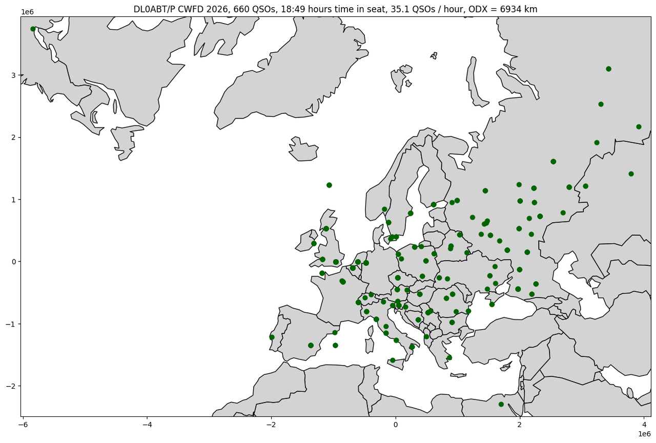
The conditions this year were not optimal. Most incoming signals had a pronounced Aurora-type hissing sound for much of Saturday evening and night. 15 m was so-so, not really open; even less was going on 10 m. During the entire contest, we reached only one station in USA and Canada, down from four last year. Furthest distance to station with a known QTH this year was 6934 km. Count of DX QSOs was up from 13 last year to 21, but given our increased total QSO number, that means that last year, we had 4.3 % DX QSOs, this year, only 3.2 %.
DXCCs we reached, and with how many QSOs:
Albania: 1
Austria: 6
Balearic Islands: 2
Belarus: 7
Belgium: 26
Bosnia-Herzegovina: 3
Bulgaria: 3
Croatia: 2
Czech Republic: 20
Denmark: 2
Egypt: 1
England: 96
Faeroe Islands: 3
Finland: 5
France: 5
Germany: 208
Greece: 1
Guernsey: 3
Hungary: 5
Ireland: 3
Italy: 20
Kaliningrad (Koenigsberg): 1
Kazakhstan: 3
(Maritime Mobile: 1)
Netherlands: 21
Norway: 1
Poland: 13
Portugal: 1
Romania: 8
Russia (Asiatic): 16
Russia (European): 88
Scotland: 13
Serbia: 7
Slovenia: 16
Spain: 7
Sweden: 9
Switzerland: 20
Ukraine: 8
United States: 1
Wales: 4
Alternatively, here is a beam map that shows the positions of our QSO partners, as far as the HamQTH API knows them:
We had 8 dupes in our log, but all of them while we were runing (i.e., calling CQ). We just accept any incoming dupes and log them again.
Raw score calculation: 1872 QSO points, 115 band/DXCC combinations (not counting “Maritime Mobile”), so raw score 215280.
N1MM comes up with 219024 as the raw score, which is 1872 x 117. So apparently, N1MM puts at least two calls into different DXCCs than does HamQTH. I did not bother to investigate.
Activity by band 🔗
The following table summarizes how much time we spent operating each band, how many QSOs resulted from such operation, the average QSO rate (in QSOs per hour) achived, and how many average QSO points per QSOs that band produced, and finally, the number of DXCCs reached on that band:
| band | hours | count | rate | avg. points | DXCC count |
|---|---|---|---|---|---|
| 10m | 0.3 | 6 | 19.1 | 2.7 | 4 |
| 15m | 2.8 | 54 | 19.3 | 2.7 | 22 |
| 20m | 5.2 | 172 | 33.2 | 2.6 | 32 |
| 40m | 5.0 | 219 | 44.0 | 2.7 | 31 |
| 80m | 3.3 | 151 | 46.3 | 3.0 | 19 |
| 160m | 2.3 | 58 | 25.3 | 3.8 | 10 |
Apparently, most stations taking part in the CW FD on 160 m were true outdoor fieldday stations.
Band strategy 🔗
How well did we distribute our operation time? Should we have stayed on any band longer?
For some idea of the answer, I calculate the number of points that we would have gone without, had we stopped operating each band a certain amount of time earlier, here measured in minutes. The rationale: If the last minutes we operated on some band result in exceptionally many end result points, it would probably have been a good idea to stay on that band longer.
The initial table and graph originally presented here was wrong. The calculation was messed up. Corrected 2026-06-12 10:15 UTC.
| 10’ | 15’ | 20’ | 30’ | 60’ | |
|---|---|---|---|---|---|
| 10m | 5112 | 9280 | 9280 | 9280 | 9280 |
| 15m | 2792 | 3022 | 3252 | 6024 | 19944 |
| 20m | 696 | 928 | 3482 | 6024 | 9330 |
| 40m | 1624 | 3016 | 3480 | 5104 | 11302 |
| 80m | 2088 | 5552 | 7852 | 10612 | 18336 |
| 160m | 4172 | 5552 | 6472 | 10356 | 14460 |
Here is that same data as a combination of one bar graph diagram per “tail time”:
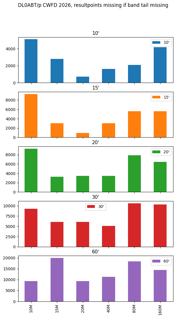
The observant reader might wonder why the numbers for 15 and 20 minutes for the 10 m band do not differ. Explanation: We stayed on 10 m for about 19 minutes. But the way we calculate this, that includes the about 6 minutes between the last QSO on the previous band and the first on 10 m. So the last 13 minutes of our presence on 10 m contain all 10 m QSOs.
This suggests we spent too much time on the “bread and butter bands” 20m and 40m. We should have invested more in 10 m, and possibly in 80 m and 160 m. It was apparently a good choice to spend comparatively little time on 15 m.
DXCCs by bands 🔗
For your amusement, here is the detailed list of which DXCCs we reached on which band:
10 m Band:
    Germany: 3
    Italy: 1
    Scotland: 1
    Spain: 1

 15 m Band:
    Balearic Islands: 1
    Belarus: 1
    Bosnia-Herzegovina: 1
    England: 13
    Faeroe Islands: 1
    Finland: 1
    Germany: 5
    Guernsey: 1
    Ireland: 1
    Italy: 3
    Kazakhstan: 1
    Poland: 1
    Portugal: 1
    Romania: 3
    Russia (Asiatic): 1
    Russia (European): 11
    Scotland: 2
    Serbia: 1
    Spain: 3
    Ukraine: 1
    Wales: 1

 20 m Band:
    Austria: 1
    Balearic Islands: 1
    Belarus: 3
    Belgium: 5
    Bosnia-Herzegovina: 1
    Bulgaria: 2
    Egypt: 1
    England: 33
    Faeroe Islands: 1
    Finland: 3
    France: 3
    Germany: 7
    Guernsey: 1
    Hungary: 1
    Ireland: 1
    Italy: 8
    Kazakhstan: 2
    Netherlands: 3
    Norway: 1
    Romania: 3
    Russia (Asiatic): 15
    Russia (European): 52
    Scotland: 4
    Serbia: 2
    Slovenia: 3
    Spain: 2
    Sweden: 2
    Switzerland: 4
    Ukraine: 4
    United States: 1
    Wales: 2

 40 m Band:
    Albania: 1
    Austria: 2
    Belarus: 2
    Belgium: 14
    Bosnia-Herzegovina: 1
    Bulgaria: 1
    Croatia: 2
    Czech Republic: 12
    Denmark: 2
    England: 25
    Faeroe Islands: 1
    Finland: 1
    France: 2
    Germany: 75
    Greece: 1
    Hungary: 2
    Ireland: 1
    Italy: 7
    Maritime Mobile: 1
    Netherlands: 14
    Poland: 5
    Romania: 2
    Russia (European): 18
    Scotland: 3
    Serbia: 3
    Slovenia: 6
    Spain: 1
    Sweden: 4
    Switzerland: 7
    Ukraine: 2
    Wales: 1

 80 m Band:
    Austria: 2
    Belarus: 1
    Belgium: 4
    Czech Republic: 7
    England: 19
    Germany: 79
    Guernsey: 1
    Hungary: 1
    Italy: 1
    Kaliningrad (Koenigsberg): 1
    Netherlands: 3
    Poland: 7
    Russia (European): 7
    Scotland: 2
    Serbia: 1
    Slovenia: 5
    Sweden: 3
    Switzerland: 6
    Ukraine: 1

160 m Band:
    Austria: 1
    Belgium: 3
    Czech Republic: 1
    England: 6
    Germany: 39
    Hungary: 1
    Netherlands: 1
    Scotland: 1
    Slovenia: 2
    Switzerland: 3
Discussion opportunity 🔗
If you want to comment or discuss this piece and have a Fediverse account, feel invited to answer my pertinent toot.
Later addition: My analysis script 🔗
At the request of a friend, I also provide my analysis script, on an as-is basis. Here it is: Auswertung.ipynb.
I provide the code in that script under the the CC0 1.0 license, that is, donate it into the public domain.
When fed with the actual ADI file, this script will disclose intimate details about our three operator’s doings, which I do not want to publish. So you’ll here get the empty version without any such details. Which unfortunately means this file does not really showcase what the analysis does, unless you run it with your own ADI file. And are lucky enough that it contains all the fields this wants; you may need to fiddle with either your file or this code to get all output.
To run the analysis, set up a Python virtual environment with the following requirements:
jupyter
notebook
matplotlib
pandas
geopandas
Cartopy
requests
adif-io
Run jupyter notebook; then a browser window should open and you can
select the file and run it.