Resonant dipoles at various heights
What is this? 🔗
This is a study of how the behavior of resonant half-wave dipoles changes when height is changed.
This is intended to be an interesting read by itself for people interested in antennas. This also serves as part of the showcase for my Python software antenna-simulation-driver, in the following sense:
- This part shows one example of what can be done with that software. We hope it will be interesting for a general audience of people interested in short-wave antennas, who may or may not be programmers.
- There is an accompanying Jupyter notebook that tells you in detail
how this was done. That part is intended for people who are
familiar with Python programming. You want to look at the
antenna-simulation-driversoftware’s showcase page if interested (maybe after briefly reading this first).
Object of study 🔗
We study resonant half-wave dipoles at different heights from 2 m above ground to 100 m above ground. We do so by running many antenna simulations (via some NEC2 variant).
Each such dipole is resonant at 7100 kHz and consists of copper wire with a diameter of 1 mm.
Dipoles are studied over two grounds: Average ground with dielectric constant of 13 and conductivity of 0.005 S/m, and city ground with dielectric constant of 3 and conductivity 0.001 S/m.
As a first step, it was determined that the resonant half-wave length of a dipole built from such wire is 20.563 m in free space.
Dipole length 🔗
It is well-known that height (somewhat) de-tunes antennas. Before doing measurements for a resonant half-wave dipole at a certain height, we first determine the precise length required for half-wave resonance at that height.
Here is this relative length, in percent of the resonant length in free space, depending on height, for average ground and city ground:
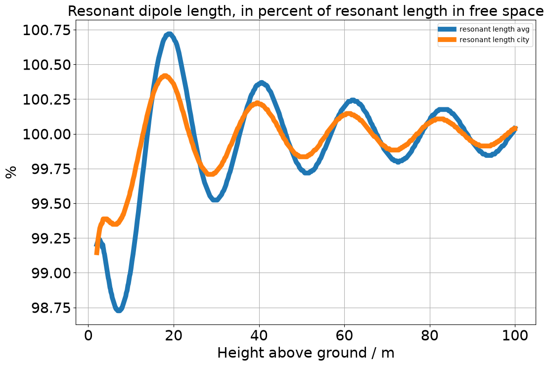
For accessibility and general karma, here is an excerpt of the same data as a textual table:
| height/m | length avg | length city |
|---|---|---|
| 2.0 | 99.20 | 99.14 |
| 3.0 | 99.21 | 99.35 |
| 4.0 | 99.10 | 99.39 |
| 5.0 | 98.91 | 99.37 |
| 6.0 | 98.78 | 99.35 |
| 7.0 | 98.73 | 99.36 |
| 8.0 | 98.75 | 99.41 |
| 9.0 | 98.86 | 99.49 |
| 10.0 | 99.03 | 99.60 |
| 12.5 | 99.64 | 99.95 |
| 15.0 | 100.26 | 100.26 |
| 20.0 | 100.69 | 100.36 |
| 25.0 | 99.96 | 99.87 |
| 30.0 | 99.52 | 99.73 |
| 35.0 | 99.93 | 100.04 |
| 40.0 | 100.36 | 100.21 |
| 45.0 | 100.12 | 100.02 |
| 50.0 | 99.74 | 99.83 |
| 55.0 | 99.86 | 99.96 |
| 60.0 | 100.19 | 100.14 |
| 65.0 | 100.16 | 100.06 |
| 70.0 | 99.86 | 99.89 |
| 75.0 | 99.84 | 99.93 |
| 80.0 | 100.10 | 100.08 |
| 85.0 | 100.16 | 100.08 |
| 90.0 | 99.94 | 99.94 |
| 95.0 | 99.85 | 99.92 |
| 100.0 | 100.04 | 100.04 |
Each of the following graphs in this blog post assumes that at each height, the half-wave dipole is used that is resonant at that height.
Sideline: computational effort 🔗
For people interested in a brief overview of the mechanics of these calculations:
- 9 simulations were needed to establish 20.563 m as the resonant dipole length in free space, using the toms748 root finding algorithm from scipy.
- 441 data points went into each of the curves: 80 of those for the heights up to 10 m (every 0.1 m), 361 for the heights up to 100 m (every 0.25 m).
- The result of the simulations were 882 data records. Each data record contains various values for the resonant dipoles at a certain height over one of the two grounds. The graphs and tables in this present blog post expose different aspects of those 882 data points.
- Most antenna simulations were used to establish the resonant length at each height. Length calculations were started from scratch at each height. It would have been beneficial to optimize by using the result of nearby heights. However, this was not done, but plain toms748 was thrown at the problem instead. A total of 11670 antenna simulations were needed with this wasteful approach. Spreading those over 4 cores (and 4 would-be cores, aka “hyperthreading”) meant all of these simulations took a little less than 8 minutes. It was judged that coding the optimization would have slowed down proceedings.
Loss 🔗
Loss changes with height. We map combined wire and ground loss, again for both average and city ground, measured in dB.
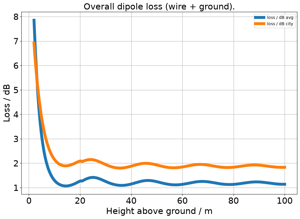
For accessibility and general karma, here is an excerpt of the same data as a textual table:
| height/m | avg | city |
|---|---|---|
| 2.0 | 7.8 | 6.9 |
| 3.0 | 5.7 | 5.6 |
| 4.0 | 4.1 | 4.6 |
| 5.0 | 3.1 | 3.8 |
| 6.0 | 2.4 | 3.3 |
| 7.0 | 2.0 | 2.9 |
| 8.0 | 1.7 | 2.5 |
| 9.0 | 1.4 | 2.3 |
| 10.0 | 1.3 | 2.2 |
| 12.5 | 1.1 | 1.9 |
| 15.0 | 1.1 | 1.9 |
| 20.0 | 1.3 | 2.1 |
| 25.0 | 1.4 | 2.1 |
| 30.0 | 1.3 | 1.9 |
| 35.0 | 1.1 | 1.8 |
| 40.0 | 1.1 | 1.9 |
| 45.0 | 1.3 | 2.0 |
| 50.0 | 1.2 | 1.9 |
| 55.0 | 1.1 | 1.8 |
| 60.0 | 1.1 | 1.8 |
| 65.0 | 1.2 | 1.9 |
| 70.0 | 1.2 | 1.9 |
| 75.0 | 1.2 | 1.8 |
| 80.0 | 1.1 | 1.8 |
| 85.0 | 1.2 | 1.9 |
| 90.0 | 1.2 | 1.9 |
| 95.0 | 1.2 | 1.9 |
| 100.0 | 1.1 | 1.8 |
Dipole impedance 🔗
Dipole impedance also varies with height.
As we exclusively deal with resonant dipoles, all impedances are purely ohmic, in other words, there is no capacitive or inductive component, or, in still other words, the impedance has no imaginary part.
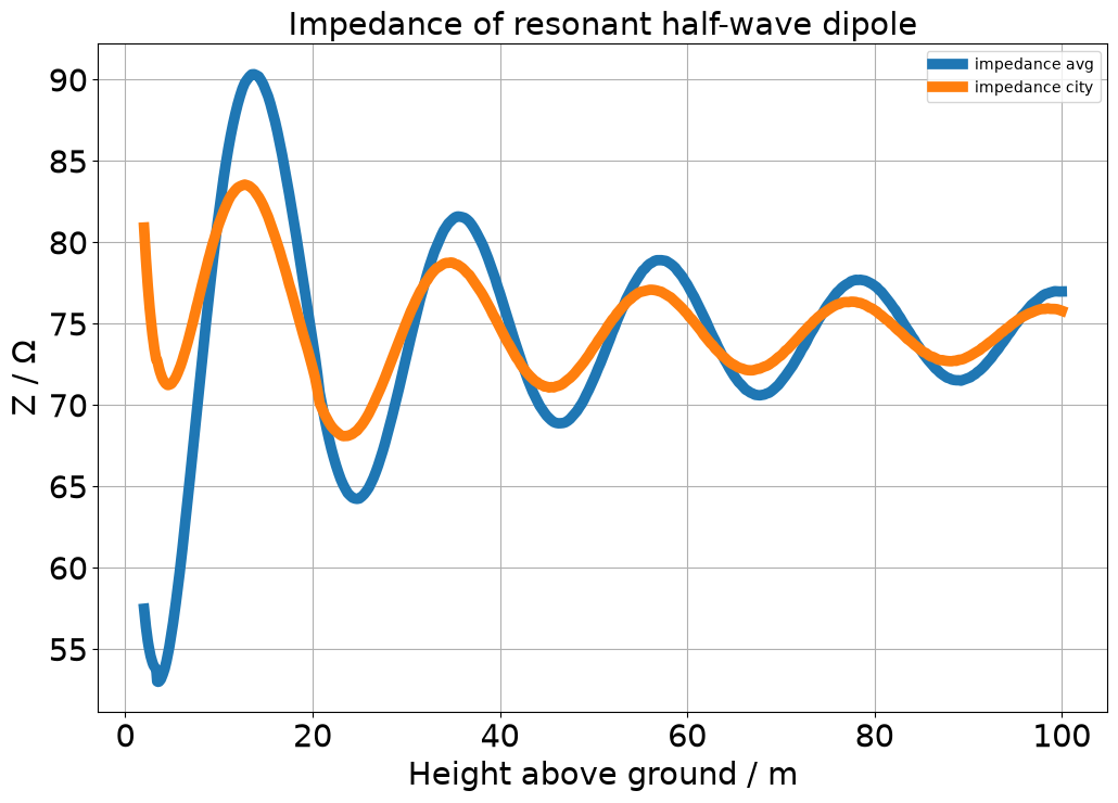
For accessibility and general karma, here is an excerpt of the same data as a textual table:
| height/m | Z/Ω avg | Z/Ω city |
|---|---|---|
| 2.0 | 57.5 | 80.9 |
| 3.0 | 54.0 | 73.9 |
| 4.0 | 53.4 | 71.6 |
| 5.0 | 56.2 | 71.4 |
| 6.0 | 60.7 | 72.6 |
| 7.0 | 66.1 | 74.6 |
| 8.0 | 71.7 | 76.9 |
| 9.0 | 77.1 | 79.2 |
| 10.0 | 81.8 | 81.1 |
| 12.5 | 89.4 | 83.5 |
| 15.0 | 89.3 | 81.9 |
| 20.0 | 74.0 | 72.3 |
| 25.0 | 64.3 | 68.6 |
| 30.0 | 72.9 | 75.1 |
| 35.0 | 81.4 | 78.7 |
| 40.0 | 76.9 | 74.8 |
| 45.0 | 69.3 | 71.1 |
| 50.0 | 71.6 | 73.5 |
| 55.0 | 78.0 | 76.9 |
| 60.0 | 77.4 | 75.6 |
| 65.0 | 71.8 | 72.5 |
| 70.0 | 71.4 | 73.0 |
| 75.0 | 76.1 | 75.8 |
| 80.0 | 77.3 | 75.8 |
| 85.0 | 73.3 | 73.4 |
| 90.0 | 71.6 | 73.0 |
| 95.0 | 74.9 | 75.1 |
| 100.0 | 77.0 | 75.8 |
Gain for a DX QSO 🔗
For DX QSOs, flat radiation is generally beneficial. Ground gain helps, too, which is very height-dependent.
We somewhat arbitrarily assume the ionosphere has an apparent height of 400 km, and we’ll reach that DX station if the first hop carries our signals back to ground 2000 km from home.
For this, our radio waves need to be emitted at an elevation of 17° above the horizon. So we ask our antenna simulation: What is the directional gain at that elevation, in dBi? We are interested in the “best” direction, perpendicular to the dipole wire. And we want to know directional gain depending on antenna height.
Here is the result:
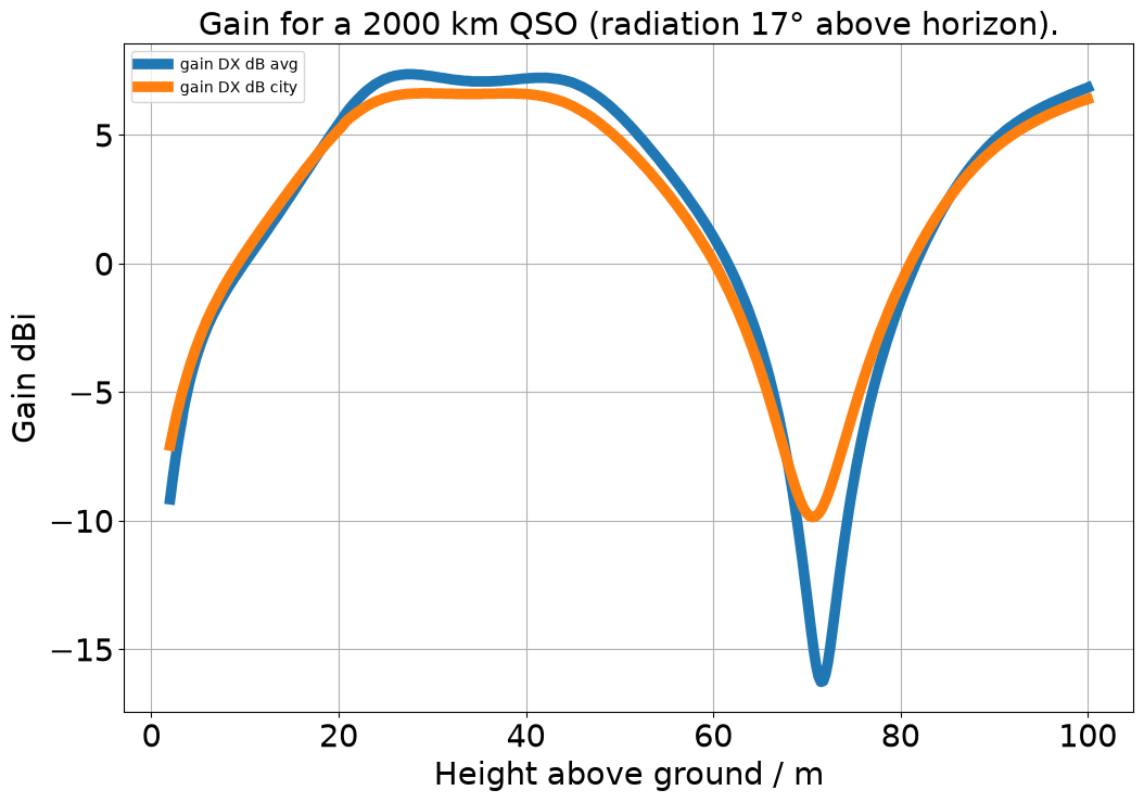
For accessibility and general karma, here is an excerpt of the same data as a textual table:
| Height/m | dBi avg | dBi city |
|---|---|---|
| 2.0 | -9.2 | -7.1 |
| 3.0 | -6.6 | -5.4 |
| 4.0 | -4.7 | -4.1 |
| 5.0 | -3.4 | -3.0 |
| 6.0 | -2.5 | -2.2 |
| 7.0 | -1.7 | -1.4 |
| 8.0 | -1.1 | -0.7 |
| 9.0 | -0.5 | -0.1 |
| 10.0 | 0.0 | 0.4 |
| 12.5 | 1.4 | 1.7 |
| 15.0 | 2.7 | 3.0 |
| 20.0 | 5.4 | 5.2 |
| 25.0 | 7.2 | 6.4 |
| 30.0 | 7.3 | 6.6 |
| 35.0 | 7.1 | 6.6 |
| 40.0 | 7.2 | 6.6 |
| 45.0 | 7.0 | 6.1 |
| 50.0 | 5.8 | 4.8 |
| 55.0 | 3.7 | 2.8 |
| 60.0 | 1.0 | 0.1 |
| 65.0 | -3.1 | -4.1 |
| 70.0 | -12.9 | -9.7 |
| 75.0 | -8.5 | -5.7 |
| 80.0 | -1.5 | -0.8 |
| 85.0 | 2.4 | 2.4 |
| 90.0 | 4.8 | 4.5 |
| 95.0 | 6.0 | 5.6 |
| 100.0 | 6.8 | 6.4 |
NVIS gain 🔗
Not everybody is interested in far-away DX stations. For the opposite, “nearly vertical incident skywave” NVIS, we need radiation straight up.
Again, the gain in that direction depends on antenna height. Here is the data:
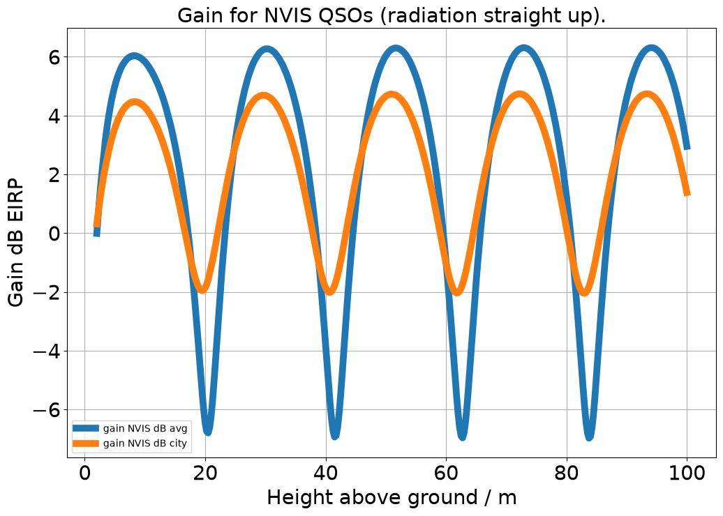
For accessibility and general karma, here is an excerpt of the same data as a textual table:
| height/m | dBi avg | dBi city |
|---|---|---|
| 2.0 | -0.0 | 0.3 |
| 3.0 | 2.4 | 1.8 |
| 4.0 | 4.0 | 2.8 |
| 5.0 | 5.0 | 3.6 |
| 6.0 | 5.6 | 4.1 |
| 7.0 | 5.9 | 4.4 |
| 8.0 | 6.0 | 4.5 |
| 9.0 | 6.0 | 4.4 |
| 10.0 | 5.8 | 4.3 |
| 12.5 | 4.9 | 3.4 |
| 15.0 | 3.0 | 1.6 |
| 20.0 | -6.5 | -1.9 |
| 25.0 | 3.1 | 3.0 |
| 30.0 | 6.3 | 4.7 |
| 35.0 | 4.4 | 2.7 |
| 40.0 | -3.8 | -1.9 |
| 45.0 | 1.0 | 1.8 |
| 50.0 | 6.0 | 4.7 |
| 55.0 | 5.3 | 3.6 |
| 60.0 | -1.0 | -1.0 |
| 65.0 | -1.7 | 0.5 |
| 70.0 | 5.5 | 4.4 |
| 75.0 | 5.9 | 4.2 |
| 80.0 | 1.3 | 0.2 |
| 85.0 | -4.8 | -0.8 |
| 90.0 | 4.6 | 3.9 |
| 95.0 | 6.2 | 4.5 |
| 100.0 | 3.0 | 1.4 |
Other sources 🔗
This ends the study of resonant half-wave dipoles of different heights.
It was done using my Python software
antenna-simulation-driver,
available via Pypi. That software does not have all “batteries
included”, it needs nec2++ to be installed. See the software’s
README
for details.
This text you just read is intended as a good, convenient entrance to
get to know one of the things the antenna-simulation-driver software
can do. If you want to know how it was done, you are invited to
download, read, and maybe run the Jupyter notebook
source that produced the
graphs and numbers (recommended name resonant_dipoles.ipynb). The
showcase page has instructions how to view and maybe
run. It also
has further examples of what else can be done with the software.
For a first glance into how this height parameter study was done, you can also try a pre-rendered version of the notebook. I find the formatting rather crappy, so I don’t fully recommend it.
Details, for the record 🔗
The study was organized as a Jupyter notebook, so besides Python 3.13,
we used the “usual suspects” installed with pip:
numpy
notebook
pandas
matplotlib
scipy
In case you need to know (you probably don’t), the versions of those
pieces of software and the dependencies pulled in by them were, in
requirements.txt format:
antenna-simulation-driver==0.3.0
anyio==4.14.2
argon2-cffi==25.1.0
argon2-cffi-bindings==25.1.0
arrow==1.4.0
asttokens==3.0.2
async-lru==2.3.0
attrs==26.1.0
babel==2.18.0
beautifulsoup4==4.15.0
bleach==6.4.0
certifi==2026.7.22
cffi==2.1.1
charset-normalizer==3.5.1
comm==0.2.3
contourpy==1.3.3
cycler==0.12.1
debugpy==1.8.21
decorator==5.3.1
defusedxml==0.7.1
executing==2.2.1
fastjsonschema==2.22.2
fonttools==4.63.0
fqdn==1.5.1
h11==0.16.0
httpcore==1.0.9
httpx==0.28.1
idna==3.19
ipykernel==7.3.0
ipython==9.16.1
ipython-pygments-lexers==1.1.1
isoduration==20.11.0
jedi==0.20.0
jinja2==3.1.6
json5==0.15.0
jsonpointer==3.1.1
jsonschema==4.26.0
jsonschema-specifications==2025.9.1
jupyter-builder==1.2.2
jupyter-client==8.9.1
jupyter-core==5.9.1
jupyter-events==0.12.1
jupyter-lsp==2.3.1
jupyter-server==2.20.0
jupyter-server-terminals==0.5.4
jupyterlab==4.6.3
jupyterlab-pygments==0.3.0
jupyterlab-server==2.28.0
kiwisolver==1.5.0
lark==1.3.1
markupsafe==3.0.3
matplotlib==3.11.1
matplotlib-inline==0.2.2
mistune==3.3.4
nbclient==0.11.0
nbconvert==7.17.1
nbformat==5.11.1
nest-asyncio2==1.7.2
notebook==7.6.2
notebook-shim==0.2.4
numpy==2.5.2
packaging==26.3
pandas==3.0.5
pandocfilters==1.5.1
parso==0.8.7
pexpect==4.9.0
pillow==12.3.0
platformdirs==4.11.3
prometheus-client==0.26.0
prompt-toolkit==3.0.53
psutil==7.2.2
ptyprocess==0.7.0
pure-eval==0.2.3
pycparser==3.0
pygments==2.21.0
pyparsing==3.3.2
python-dateutil==2.9.0.post0
python-json-logger==4.2.0
pyyaml==6.0.3
pyzmq==27.1.0
referencing==0.37.0
requests==2.34.2
rfc3339-validator==0.1.4
rfc3986-validator==0.1.1
rfc3987-syntax==1.1.0
rpds-py==2026.6.3
scipy==1.18.0
send2trash==2.1.0
setuptools==82.0.1
six==1.17.0
soupsieve==2.9.2
stack-data==0.6.3
terminado==0.18.1
tinycss2==1.5.1
tornado==6.5.8
traitlets==5.16.1
typing-extensions==4.16.0
tzdata==2026.3
uri-template==1.3.0
urllib3==2.7.0
wcwidth==0.8.2
webcolors==25.10.0
webencodings==0.6.1
websocket-client==1.9.0
Discussion opportunity 🔗
If you want to comment or discuss this piece and have a Fediverse account, feel invited to answer my pertinent toot.